Quantum computing companies have ambitious physical qubit headcount targets for the next decade, and roadmaps from all qubit modalities depend on modularity to scale beyond 1,000+ qubits (link to qubit company roadmaps at the bottom of this age).

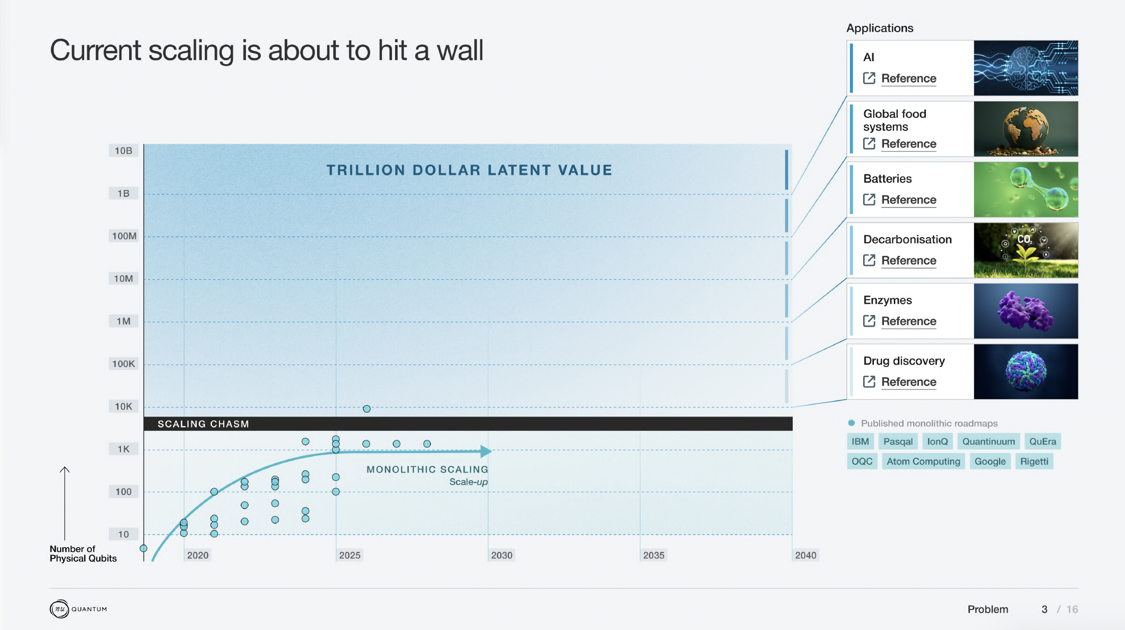
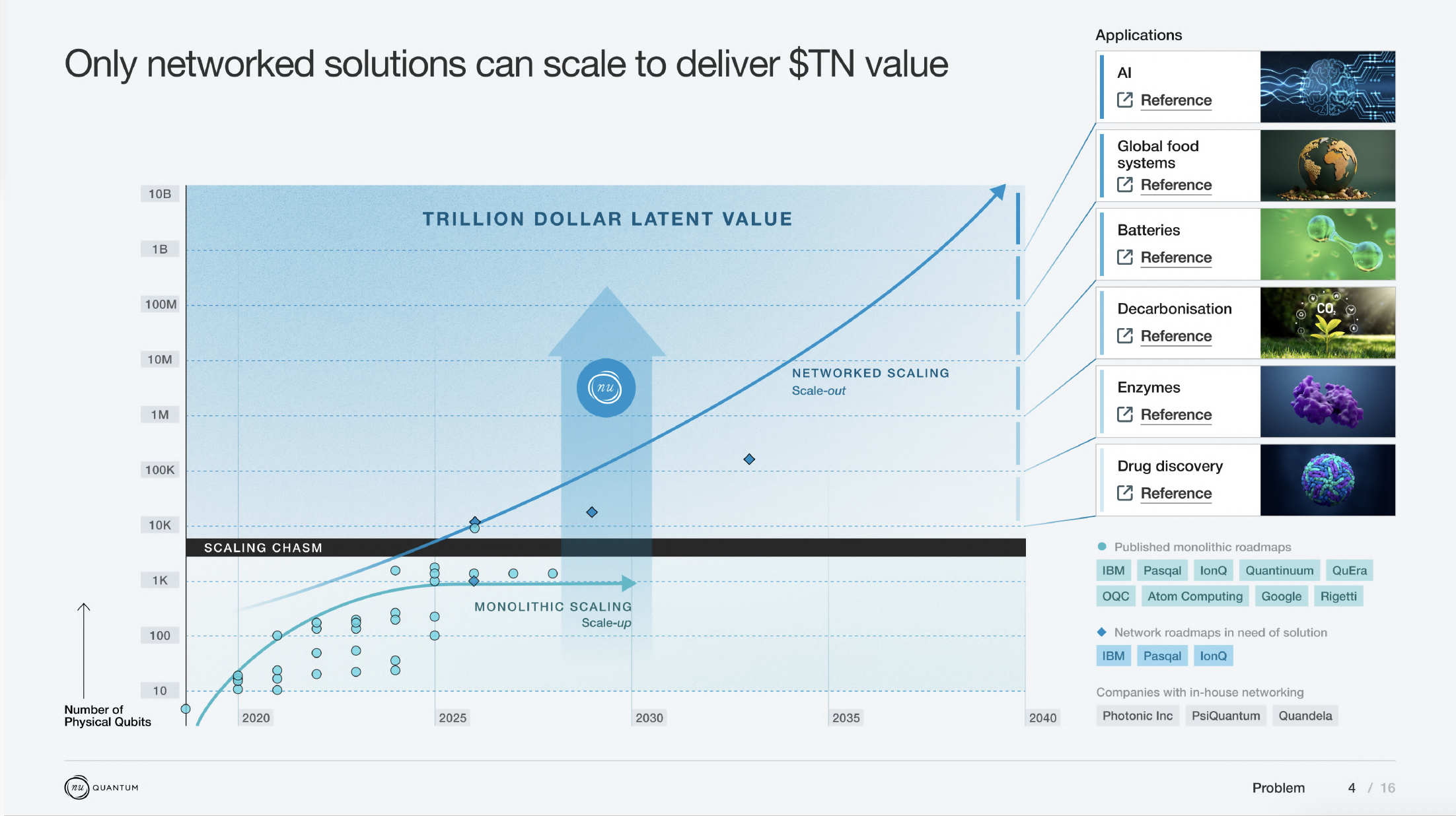
‍In this section, we delve into why scaling quantum computers monolithically is so hard, as well as why scaling processors to higher qubit counts is necessary to achieve fault-tolerant quantum computing.

Why Scaling is Hard

Figures of Merit for Quantum Computers

There are four main benchmarks for quantum computing hardware:

• Qubit number: addressed below
• Fidelity of local operations: There has been huge progress in the field on this metric. The current state-of-the-art in qubit fidelity is held by trapped-ion qubits. Oxford Ionics’ 2024 results demonstrate quantum-logic operations at the 10⁴ error level (http://arxiv.org/pdf/2407.07694). This marks an order of magnitude improvement over previous results (Quantinuum’s 2023 results in  https://journals.aps.org/prx/abstract/10.1103/PhysRevX.13.041052).

{{fidelity-of-local-operations="/rich-text-content/tables/the-scaling-chasm-for-quantum-computing"}}

• Qubit connectivity: whether any qubit can be entangled with any other qubit, or with a particular subset of its neighbours, e.g. nearest neighbours. With atomic modalities, there has been huge progress. Creating all-to-all connectivity by ‘shuttling’ and reordering qubits is well established in one dimension (i.e. ion chain). Shuttling in two dimensions (i.e. ion grids) is actively pursued  to minimise the time it takes to create all-to-all connectivity (see for e.g. Quantinuum’s results in https://arxiv.org/pdf/2403.00756). With the shuttling approach, the overhead of shuttling increases with distance and system size, and there will be a point where Nu Quantum’s optical interconnects are more favourable than a brute-force QPU scaling to realise this long-range connectivity. As both technologies are constantly evolving, it is hard to specify where the crossover will be; but Nu Quantum’s estimate is that this will happen around 100-1000 physical qubits. This estimate is based on the fact that, our optical links will operate at  ~10-50 kHz in the near term (5 years) whilst a single cycle that includes sorting and shuttling operates at ~ 0.1 kHz at N~50 qubits  (or ~2 kHz for one long-range link).
• Qubit ‘lifetime’: The coherence time of the qubit dictates the number of quantum operations that can be performed and limits ‘waiting times’ beyond which the quantum state cannot be used for computation.

To date, quantum hardware has not met computational needs on all metrics simultaneously. In general, ion traps are challenging to scale to very large qubit counts, superconducting devices have very restricted connectivity and lifetimes, neutral atoms experience high loss rates and gate errors and solid-state qubits (such as defect centers or quantum dots) are not as mature (challenging to scale, currently operate at very low fidelities).

‍

The need for Quantum Error Correction

All of the most valuable use-cases of quantum computing need Fault Tolerant computers, with hundreds to thousands of logical qubits, and with errors below 10^-6.  Because we expect qubits to always be noisier (lower fidelity) than this, the industry has developed something called Quantum Error Correction (QEC).

The QEC process turns a noisy Quantum Computer into one that is able to carry out many more logical operations without errors. This is what we mean with ‘Fault Tolerant Quantum Computers’. As with classical randomised algorithms, the chance of experiencing a logical fault at any point in a algorithm needs to be low, but not zero, so a small number of repeats can guarantee correctness.

A number of noisy physical qubits (displaying a certain gate fidelity), are used to encode one almost-perfect logical qubit (displaying higher fidelity that the physical qubits it is made out of).

• QEC is not a magic wand though - the physical qubits need to have fidelities above a threshold for QEC to do anything at all. The higher the starting fidelity, the better—the QEC performance is exponentially sensitive to physical error rates. For example, Google’s most recent surface code study predicts a 2x improvement in physical error would result in a 1000x improvement in logical lifetime (Quantum error correction below the surface code threshold, Google Quantum AI, https://arxiv.org/abs/2408.13687).

QEC protocols reduce errors by introducing redundancy, reducing the number of logical qubits by a polynomial factor in order to improve circuit depth by an exponential factor. The ratio of physical qubits required against the number of logical qubits provided (physical : logical) is a benchmark called the encoding rate.

‍

QEC Codes

There are multiple QEC codes that can be used. The qubit ratio depends on the code. The codes one can use on a particular physical system depends on the qubit connectivity and gate fidelity of that system.

Surface Code

Up until recently, the main QEC code used by the industry was the Surface Code. The Surface Code is very well understood. It assumes a ‘nearest neighbour’ connectivity between qubits, which is the most common in superconducting qubit systems.

• However, it is not very efficient at scale and for most large systems (i.e. if you are trying to build a very big computer), the physical-to-logical qubit ratios are 1000:1. This is extremely daunting for qubit vendors!
• Restricting QEC codes to using local interactions on a 2D-chip means that there aren’t better ways of doing QEC and that the Surface code is optimum (https://journals.aps.org/prl/abstract/10.1103/PhysRevLett.104.050503). To lower the QEC overhead, we need non-local interactions, and non-planar QEC codes (https://journals.aps.org/prl/abstract/10.1103/PhysRevLett.129.050505).

Non-planar codes

In the last two years, new QEC codes have appeared that are 100x more efficient (such as qLDPC codes), with physical-to-logical qubit ratios between 100:1 and 10:1 (qLDPC, Hyperbolic). Highly-efficient codes require long range connections, over and above the requirements of the surface code. Achieving flexible connectivity is challenging for current qubit systems that aim to be uniformly tiled to scale. Nu Quantum’s optical networking supports the requirements of efficient QEC codes.

Networked quantum clusters can be specialised to offer exactly the sparse, long range connectivity needed for the best performing quantum codes. Further, switchable networks are capable of dynamically transforming the connectivity of the network at runtime, offering access to powerful global transformations on the quantum state that enable access to faster logical clock speeds or more compact algorithms.

The requirements for interconnect fidelity are significantly lower than the requirements for local fidelity, if the QEC code and computer are co-designed. A recent preprint found a 10x improvement in surface code infidelity tolerance for optical links bridging neighbouring large neutral-atom arrays. We have found a equivalent 10x improvement in infidelity tolerance for highly-efficient hyperbolic codes constructed from ion traps of demonstrated scale.

Depending on the QEC code used, the number of physical qubits required to tackle the tasks described in Why Build Quantum Computers? are a 1000x or a 100x multiplier on the number of logical qubits needed for the particular algorithm.

The most near-term problem we know solvable on a Quantum Computer that is valuable and not solvable otherwise requires ~52 Logical Qubits. This leads to a physical qubit requirement of between 5,200 and 52,000 as a threshold for utility.

At the other end of utility, one of the most well-understood use-cases requiring a large number of logical qubits is breaking RSA encryption using Shor’s algorithm. This requires ~7000 logical qubits with very high fidelity. Proposed planar architectures requires **20M qubits** to break RSA due to the inefficiency of the Surface Code at scale. Bringing down the requirement on number of physical qubits required to tackle this use-case would have tremendous impact - this is precisely what a network architecture, enabling more efficient QEC codes, can make possible.

‍

Limitations to monolithic scaling

Why is it impossible to scale to tens of thousands or millions of physical qubits whilst maintaining very high fidelities (99.99%) in a single QPU?

Physical limitations

These are limitations that come from the extreme environmental and infrastructural needs required to isolate, control and operate qubits.

• Superconducting Qubits: require milikelvin temperatures. Each qubit requires a dedicated microwave control line which carries a thermal load. Dilution refrigerators are not able to cope with more than ~ a thousand qubits. With innovations in cryogenic technology and microwave lines or cryogenic control, this could go up to about 10,000 in the next 10-20 years.
• Trapped Ion Qubits. The ability to carry out gates between ions relies on the Coulomb force, and so they need to be physically close.
  • Linear trap architectures are understood to not scale beyond 50-100 qubits
  • QCCD architectures, where you shuttle and reorder qubits to achieve all-to-all connectivity, are seen to potentially scale to a thousand qubits. Oxford Ionics even forecasts 10,000 qubits on 1225 mm² chip  (http://arxiv.org/pdf/2407.07694). However the cycle time of these machines may be quite slow for quantum applications.
• Neutral Atom Qubits. Limited by laser power and field of view of a microscope.
  • Limit understood to be at around 10,000 qubits.

Chip size limitations

The analyst firm GQI made the following assessment:

"The first step to scaling up a system is to seek to put the maximum number of qubits on a single chip. At the most basic level this is set by the size of the qubit unit cell versus the fabrication die size."

GQI believes we need to be cautious about simply adopting design rules and assumptions from conventional semiconductor fab to quantum applications. The tradeoffs may be different, particularly because the dynamics of Moore’s law and process node miniaturization do not automatically apply.  However we recommend caution when die sizes above 800mm2 are assumed.

The significance of individual chip sizes is that they set the maximum level of qubit scaling that can be achieved using only native connectivity.  Additional factors affect module size such as the thermal cooling power available. This is particularly impacted by control plane requirements.

Given that our quantum plane chips will in most cases have a qubit count less than we require for large scale systems, ways to share entanglement across chips are essential. This naturally supports modular scaling. However, it is also important to understand how such technologies also impact overall connectivity and the QEC codes that may ultimately be employed.

Yield and Performance limitations

{{yield-and-performance-limitations="/rich-text-content/tables/the-scaling-chasm-for-quantum-computing"}}

The above maximum scaling numbers are theoretical maxima. However, there are real-world engineering considerations that temper the above numbers.

Fidelity is crucial - and a Quantum Computer is as good as its worse error (2-qubit gate or SPAM or decoherence during shuttling). When pushing systems to the limit, the yield will go down, and the performance of the system will go down. This is why no qubit company roadmap actually assumes scaling monolithically to millions of qubits.

‍

‍